Live Earthquake | 실시간 지진 지도
This is a live earthquake visualization dashboard connected to the USGS earthquake API (no key required, CORS-enabled).
Filters: Combine time range (Past Hour / Day / 7 Days / 30 Days) with minimum magnitude (All M1.0+ / M2.5+ / M4.5+ / Significant), mapped directly to USGS's actual feed URLs ({threshold}_{period}.geojson).
World Map: Each earthquake is shown as a dot sized and colored by magnitude (green → yellow → orange → red → purple). Clicking a dot auto-scrolls to it in the list below.
Magnitude Distribution: A bar chart showing how many quakes fell into each magnitude range (<2 / 2–3 / 3–4 / 4–5 / 5–6 / 6+).
Depth vs. Magnitude: A scatter plot showing the relationship between magnitude and depth (deeper quakes plot lower, stronger quakes plot further right).
Recent Earthquakes list: Sorted by magnitude, showing location, depth, and time elapsed, with click-to-highlight on the map.
Summary cards: Total quake count, largest magnitude, average magnitude, and average depth.
👁 7
👍 0
♻ 0
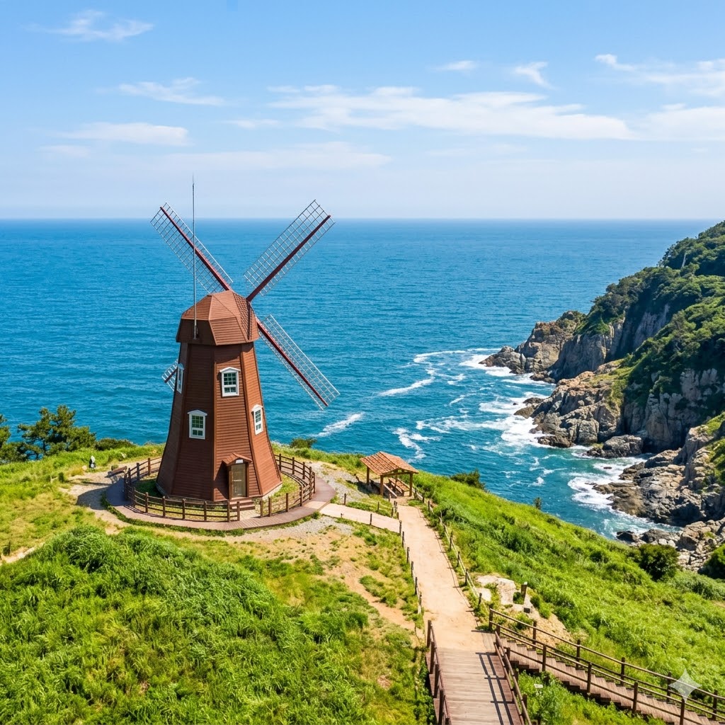
World Weather | 세계의 날씨
World Map: Shows each city on a world map drawn with d3-geo, colored by current temperature (blue = cold → red = hot). Clicking a city displays it in the detail panel.
City Chips: Lists all cities as chips along with their current temperature, so you can quickly select one.
Current Weather detail: Shows the selected city's current temperature, feels-like temperature, humidity, and wind speed with icons, along with a 24-hour temperature graph for today and a 7-day high/low temperature bar chart.
Compare Cities: Compares the current temperature of all cities in a sorted bar chart.
Language selector: In the top right, you can switch between English / Français / 한국어 / 日本語 / 中文 — this switches all UI text, weather condition descriptions, and even city names.
👁 10
👍 0
♻ 0
🤖 Robotics
🦾 Tab 1 — Robot Arm
Visualises forward and inverse kinematics for a 3-DOF robotic arm. IK is solved in real time using the CCD (Cyclic Coordinate Descent) algorithm. Drag the white circle target and the arm follows; link lengths and IK iteration count are adjustable via sliders. Includes Auto Demo mode (circular trajectory) and Draw Path mode (trace a custom path with the mouse).
🧭 Tab 2 — Path Planning
Animates three pathfinding algorithms — A*, RRT, and Dijkstra — on an interactive grid. Click the canvas to toggle obstacles, and hit Random Maze to generate a randomised layout. Explored cells are highlighted in blue and the final path in green, both updating in real time.
👁 Tab 3 — Computer Vision
Processes four moving objects through five vision pipeline modes: RGB (raw), Grayscale (luminance conversion), Edge (Sobel edge detection), Depth (false-colour depth estimation map), and Detect (bounding boxes with confidence scores). Drag any object to see the detection respond live.
🧠 Tab 4 — Neural Control
Three control system demos in one tab. PID Balance: an inverted pendulum with tunable Kp, Ki, and Kd gains. RL CartPole: a reinforcement learning agent balancing a pole, with the policy network visualised in real time. Biped Walker: a two-legged gait driven by a Central Pattern Generator (CPG). Click the canvas to move the PID setpoint.
🌐 Tab 5 — Swarm
Boids-based swarm robotics simulation. Three steering forces — Separation, Alignment, and Cohesion — are independently tunable via sliders. Four behaviour modes: Flock (free flocking), Forage (click to place food targets), Formation (robots self-organise into a ring), and Explore (random exploration). Obstacle avoidance is built in throughout.
👁 9
👍 0
♻ 0

표절 검사 도구
📊 유사도 점수
4가지 알고리즘의 가중 합산으로 최종 점수를 산출합니다. Ring 게이지 + 색상 판정 5단계.
코사인 유사도 (45%) — TF-IDF 벡터 간의 각도. 문서 길이와 무관
자카드 지수 (20%) — 공유 어휘 / 전체 고유 어휘 비율
바이그램 중복 F1 (20%) — 2단어 구문 일치율. 패러프레이징 탐지에 효과적
트라이그램 중복 F1 (15%) — 3단어 구문 일치율. 직접 복사의 강력한 지표
🔬 5가지 시각화 탭
📝 단어 비교 — 두 문서를 나란히 표시하고 단어별로 색상 구분
🔴 빨강 = 정확 일치 / 🟡 노랑 = 어간 일치 (패러프레이징) / 🟢 초록 = 고유 단어 / 회색 = 불용어
📐 벡터 공간 — TF-IDF 벡터를 2D로 투영해 단어를 점으로 시각화. 문서 A/B의 중심 벡터를 원점에서 화살표로 표시하고 두 벡터 사이의 각도(θ) 실시간 표시
📏 코사인 각도 — 단위 원에 두 문서 벡터를 그려 각도로 유사도를 직관적으로 표현. 공통 단어별 A/B TF-IDF 가중치 바 차트 제공
🧩 N-gram 히트맵 — 1/2/3-gram 전환 버튼으로 단어·2단어·3단어 구문 단위의 일치 여부를 격자로 시각화. 빨강 = 공유 / 파랑 = A 전용 / 주황 = B 전용
📊 단어 빈도 — 양쪽 문서의 TF-IDF 상위 단어를 바 형태로 비교. 공통 단어는 빨강으로 표시
🌐 언어 지원
영어 — TF-IDF, 불용어 제거, 접미사 기반 어간 추출 (ing/tion/ness 등)
한국어 — 어절 분리 + 조사·어미 제거 (에서/으로/합니다 등 40여 개), 1글자 및 접속사 불용어 처리
언어 자동 감지 (한글 문자 수 vs 영문자 수 비교)
BMI Calculator
⚖️ Measurement Input
Metric / Imperial toggle — instantly converts between kg·cm and lbs·ft·in
Slider + number input, two-way sync — moving the slider updates the number box and vice versa
Age input and biological sex selection (used as a reference for healthy ranges)
📊 BMI Gauge
Semi-circular analogue gauge — the needle rotates smoothly to match the BMI value via CSS transition
Five colour zones: Blue (underweight) → Green (normal) → Yellow (overweight) → Orange (obese I) → Red (obese II+)
Active category is highlighted; all others are dimmed
📐 Body Metrics Panel
Height (m), weight (kg), BMI, and category displayed in real time
Ideal weight range bar (WHO standard BMI 18.5–24.9) with a marker showing current weight position
Automatically calculates how much weight to lose or gain to reach the ideal range
💡 Health Guidance (4 tips per category)
Underweight — increase caloric intake, strength training, protein at every meal, rule out underlying causes
Normal — maintenance strategies, exercise routine, balanced diet, sleep
Overweight — 500 kcal daily deficit, walking, reduce ultra-processed food, hydration
Obese I — see a doctor, 5–10% weight loss impact, portion control, stress management
Obese II+ — medical supervision, metabolic assessment, GLP-1 medications, build a support network
📋 Reference Information
WHO BMI Classification (2004) explained
Separate guidance for Asian populations (overweight ≥ 23, obese ≥ 27.5)
Medical disclaimer noting BMI is a screening tool, not a diagnostic measure
👁 22
👍 0
♻ 0
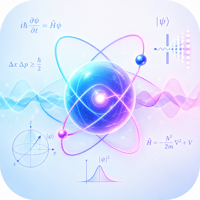
🔭 3D Solar System Explorer
A full 3D Solar System Explorer!
Controls
Drag — Rotate the viewpoint (mouse and touch both supported)
Scroll — Zoom in and out
Click a planet — Focus on that planet and open its detail info panel
Bottom pill buttons — Jump directly to any planet instantly
Top toggles
Orbits — Show or hide the orbital ellipses
Labels — Planet name labels (also shown on mouse hover)
Asteroid Belt — 320 particles filling the asteroid belt between Mars and Jupiter
▶ Play / ⏸ Paused — Freeze or resume time
Bottom sliders
Time speed — Adjust orbital speed from 0× to 5×
Zoom — Zoom level from 0.3× to 4×
Per-planet details
☀️ Sun — Triple-layer corona glow with animated sunspot texture
🌍 Earth — Continent silhouettes with a Moon orbiting in real time
🪐 Saturn — Three-layer ring system with perspective shift as the viewing angle changes
🔴 Jupiter — Horizontal cloud bands with the Great Red Spot
All planets — Full 3D sphere shading with highlight and shadow passes
Focused planet — Orbital progress arc shown as a HUD overlay
Info panel — Click any planet to display its diameter, mass, distance from the Sun, day length, year length, moon count, temperature range, surface gravity, and a key fact.
👁 31
👍 0
📟 Arduino kit
An eight-project Arduino simulator! Every project includes real Arduino code, a live circuit diagram, and a Serial Monitor at the bottom.
💡 LED Blink — The "Hello World" of hardware. A 220Ω resistor and LED circuit, digitalWrite(13, HIGH/LOW) code, and a PWM timing diagram all run simultaneously.
🔘 Button & LED — A live visualisation of INPUT_PULLUP. Click the button to light the LED, and see the inverted logic (LOW = pressed) explained in context.
🌓 PWM Fade — Controls LED brightness with analogWrite(9, 0–255). The PWM waveform and duty cycle update in real time as the LED breathes.
🌡️ Analog Sensor — Turn the potentiometer dial to read ADC values from 0 to 1023, then watch map() rescale them to the PWM range (0–255). Includes a voltage divider explanation.
⚙️ Servo Motor — Control the servo with an angle slider. The relationship between PWM pulse width (0.5ms – 2.5ms) and output angle is visualised live.
🎨 RGB LED — Mix any colour with the R, G, and B sliders. Press AUTO for an automatic rainbow cycle. A colour wheel is shown alongside.
📡 Ultrasonic Sensor — Shows how the HC-SR04 works with a TRIG/ECHO timing diagram. Verify the formula cm = round-trip time (µs) / 58 directly.
🚦 Traffic Light — Demonstrates a Finite State Machine (FSM). The RED → RED+YELLOW → GREEN → YELLOW cycle runs alongside a live state-transition diagram.
👁 43
👍 1
Physics | Double Pendulum
🌌 Gravity Well — Hold the mouse button to spawn a second gravity source and watch particles shift their orbits. A real-time visualisation of Newton's Law of Universal Gravitation.
🔵 Double Pendulum — Two pendulums starting from nearly identical conditions trace completely different paths over time. An intuitive demonstration of the Butterfly Effect at the heart of chaos theory.
〰️ Wave Interference — Renders constructive and destructive interference patterns from two wave sources in real time. Drag either source to reposition it.
🪨 Sand Pile — Click and drag to pour sand and watch the Angle of Repose form naturally as grains settle into a self-organised slope.
✨ Lissajous Curve — Adjust the X/Y frequency ratio and phase to draw circles, figure-eights, pretzels, and more. The same principle behind oscilloscope waveform analysis.
🧲 Magnetic Field — Drag the N/S poles to new positions and watch the field lines instantly reform around them.
👁 62
👍 1
Solar System | Cosmic Time
🪐 Orrery
Real-time orbital simulation using logarithmic distance scaling. Click any planet to reveal its age, formation date on the Cosmic Calendar, orbital period, surface temperature, gravity, and an age-bar showing what percentage of the Universe's lifetime it has existed. Sliders control simulation speed, orbit ring opacity, and planet display scale. Saturn's rings and the Moon's orbit are rendered separately.
⏳ Cosmic Clock
Carl Sagan's Cosmic Calendar — 13.8 billion years compressed into a single year. A circular clock face marks key events from the Big Bang to the present: galaxy formation, the Sun igniting, Earth's birth, the Cambrian Explosion, dinosaurs, and the appearance of humans. The current real-world time updates live at the centre every second.
📅 Timeline
22 major cosmic events from the Big Bang to the present, laid out on a horizontal timeline. Labels alternate above and below the axis for readability. A scrollable side panel provides a detailed description of each event alongside its age in billions of years.
⚖️ Age Compare
Horizontal bar chart comparing the ages of the Universe, the Milky Way, the Sun, all eight planets, and the Moon. Each bar shows how many billion years after the Big Bang the object formed, its age as a percentage of the Universe's total age, and its equivalent position on the Cosmic Calendar in months.
🌡 Properties
Five switchable data modes — Size, Temperature, Gravity, Density, and Moon count — displayed as bubbles positioned along a logarithmic distance axis. Bubble size and colour update instantly when switching modes, letting you compare the physical extremes of the Solar System at a glance.
👁 2
👍 0
♻ 0
날씨 정보
🗺 도시 현황 — 서울·부산·인천·대구·대전·광주·수원·울산·제주·춘천 10개 도시의 실시간 날씨 카드. 기온별 색상 구분(빨강=더움/노랑=따뜻/초록=쾌적/파랑=선선), 날씨 아이콘 애니메이션. 폭염·천둥·고습도 경보 자동 표시.
📊 상세 분석 — 선택 도시의 64px 대형 기온 표시, 7가지 세부 지표(체감·습도·기압·바람·풍향·구름·가시거리). 시간별 예보 스크롤, 24시간 기온 추이 그래프, 강수 확률 막대 차트, 바람 세기 면적 차트.
📅 주간 예보 — 7일 예보 리스트(최저/최고 온도 바 포함), 주간 최저·최고 기온 꺾은선 그래프(빨강=최고, 파랑=최저), 일별 강수 확률 막대 차트.
🗾 날씨 지도 — Canvas로 그린 한국 지도 위에 도시별 기온 색상 점 표시. 마우스 오버 시 툴팁, 클릭 시 도시 선택. 수도권·강원·충청·경상·전라·제주 지역별 평균 기온 요약.
⚖️ 도시 비교 — 기온 순위 테이블(금·은·동 메달 배지), 기온·습도 수평 막대 차트 비교.
👁 3
👍 0
♻ 0
나는 어떤 직장인 유형일까 ?
1. 인트로: 소개 + 소요시간/문항수/유형수 안내
2. 퀴즈: 12문항(4가지 축 × 3문항씩) — 업무방식(체계형/즉흥형), 관계(협업형/독립형), 의사결정(논리형/공감형), 동기(목표형/의미형)
3. 결과: 16가지 유형 중 하나를 판정해 3가지 방식으로 시각화
a. 유형 카드 (아이콘·이름·설명·키워드 뱃지)
b. 레이더 차트 (4축 성향을 SVG로 시각화)
c. 축별 비교 막대 (예: 체계형 67% vs 즉흥형 33%)
d. "잘 맞는 동료" 궁합 텍스트(반대 유형 자동 매칭)
👁 8
👍 0
♻ 0
AI 에이전트 대시보드
AI Agent Dashboard — 실시간 에이전트 모니터링, 태스크 큐, 성능 지표, 이벤트 로그를 한 화면에. 인터랙티브 시뮬레이션으로 데이터가 살아있는 느낌.
시각화 구성:
1. 상단 KPI 카드 — 활성 에이전트, 처리 태스크, 성공률, 평균 응답시간
2. 에이전트 상태 그리드 — 각 에이전트별 상태/부하/모델 표시
3. 실시간 태스크 큐 — 진행중/대기/완료 태스크 리스트
4. 성능 차트 — Canvas 기반 라인 차트 (응답시간 추이)
5. 이벤트 로그 — 타임스탬프 + 레벨별 실시간 스트리밍
6. 모델 사용 분포 — 도넛 차트
👁 6
👍 0
♻ 0
간편 칸반보드
4개 보드 프리셋
🛠 개발 프로젝트 — 백로그·할일·진행중·검토·완료 5단계 컬럼
📣 마케팅 — 아이디어·기획·실행중·완료
👤 개인 할일 — 받은함·오늘·이번주·완료
⚡ 스프린트 — 백로그·진행중·테스트·완료
3가지 뷰
⊞ 보드 뷰 — 드래그 앤 드롭으로 카드를 칼럼 간 이동. 칼럼별 완료 진행 바 표시
☰ 리스트 뷰 — 테이블 형태로 전체 카드를 한눈에 비교. 행 클릭으로 수정 가능
📅 타임라인 뷰 — 마감일 기준 간트 차트. 오늘 기준선(빨간 선) 표시
📊 통계 뷰 — 전체 현황 KPI, 우선순위 도넛 차트, 칼럼별·담당자별 바 차트, 평균 진행도, 태그 분포
카드 기능 — 제목·설명·담당자·마감일·우선순위·진행도(%)·칼럼·태그 설정. 마감 초과 시 빨간 경고 표시
필터 & 검색 — 우선순위별 필터, 마감초과 필터, 실시간 텍스트 검색
👁 4
👍 0
♻ 0
🐠 Drift Aquarium
Inside the tank: soft light beams, 5–6 swimming bioluminescent fish, swaying seaweed, rising bubbles
Mood light effect: a soft glow that spreads onto the wall behind the tank (choose from Deep Sea teal / Coral Dusk amber / Moonlight purple / Neon Reef pink)
Interaction: tap the water to send out ripples and draw the fish toward that spot; use the brightness slider to adjust the mood light intensity
👁 7
👍 0
♻ 0
The Water Cycle
This is an English HTML that visualizes the water cycle in four different ways.
01 · Live Scene — In a landscape with a sun, ocean, mountain, and river, this shows a real-time animation of water vapor rising from the ocean as the sun heats it, clouds condensing and eventually saturating to release rain over the mountain, and the river flowing back down to the ocean. The "Sun intensity" slider lets you control the evaporation rate.
02 · Process Loop — A circular diagram connecting Evaporation → Transpiration → Condensation → Precipitation → Infiltration → Runoff/Collection. Clicking each stage displays its description.
03 · Earth's Water — A donut chart showing the actual distribution of Earth's water (oceans 96.5%, glaciers 1.74%, groundwater 1.69%, surface water 0.06%, atmosphere 0.001%), based on approximate USGS figures.
04 · Stages — Each of the six stages is explained in a card with an accompanying icon.
나의 성격 유형은?
MBTI 스타일의 16문항 성격 진단 퀴즈이며, 결과를 3가지 방식으로 시각화한 한글 HTML입니다.
퀴즈 진행: 외향-내향(EI), 감각-직관(SN), 사고-감정(TF), 판단-인식(JP) 4개 축에 대해 각각 4문항씩, 총 16문항을 5단계(전혀 아니다~매우 그렇다)로 답하면 자동으로 다음 질문으로 넘어갑니다. 진행률 바와 이전 질문으로 돌아가기 기능도 있습니다.
결과 화면
- 큰 4글자 타입: 예) ENFP처럼 결과 유형을 색상별로 크게 표시
- 01 · 축별 스펙트럼 바: 각 축에서 어느 쪽으로 몇 % 기울었는지 마커와 함께 시각화
- 02 · 선호 강도 레이더: E/I/S/N/T/F/J/P 8개 축을 방사형으로 펼쳐 성향의 뚜렷함을 보여줌
- 03 · 유형 한 글자씩 설명: 각 글자의 의미와 특징을 카드로 정리
하단에 "MBTI는 학술적으로 완전히 검증된 심리 진단 도구가 아니다"라는 안내 문구를 넣어 오해를 방지했습니다.
👁 7
👍 0
♻ 0

🎛️ Synthesizer
🎹 Keyboard Performance
Play by clicking or touching the piano keys at the bottom of the screen
Keyboard shortcuts: A S D F G H J K L ; ' (white keys) / W E T Y U O P (black keys)
📊 4 Visualizations (Tab Switching)
Waveform — Real-time waveform with dry/wet two-layer overlay
Spectrum — FFT frequency spectrum bar chart with color gradient
Lissajous — XY oscilloscope Lissajous pattern (stereo phase visualization)
Particles — Sound energy-reactive particles + circular ring visualizer
🎛️ Control Panel
Oscillator — Sine / Square / Saw / Triangle waveforms + Detune / Volume / Octave knobs
Filter — LP / HP / BP / Notch + Cutoff / Resonance
ADSR Envelope — Attack / Decay / Sustain / Release
LFO — Rate / Depth, toggle ON/OFF
Effects — Reverb / Delay (Mix, Time, Feedback)
Presets — 6 instant presets: Lead / Pad / Bass / Pluck / Organ / Bell
👁 15
👍 0
♻ 0
식단 영양소 분석
식단의 영양소 비율을 4가지 방식으로 시각화한 한글 HTML입니다. 기본 예시 식단(하루치)이 미리 채워져 있어 바로 결과를 확인할 수 있습니다.
음식 추가/목표 설정: 15가지 음식 DB에서 골라 끼니(아침/점심/저녁/간식)와 섭취량(g)을 입력해 추가하고, 하루 목표 칼로리·탄단지·식이섬유·나트륨도 직접 조절할 수 있습니다.
01 · 탄단지 칼로리 비율 도넛: 무게가 아닌 칼로리 기여 비율(탄수화물·단백질 4kcal/g, 지방 9kcal/g 기준)로 정확하게 계산해 도넛 차트로 보여줍니다.
02 · 끼니별 영양소 구성: 아침·점심·저녁·간식 각각의 칼로리가 탄수화물/단백질/지방으로 어떻게 구성되는지 스택 바로 비교합니다.
03 · 목표 대비 레이더 차트: 칼로리·탄수화물·단백질·지방·식이섬유·나트륨 6개 항목을 목표치의 100% 기준선과 함께 방사형으로 보여줍니다.
04 · 요약 카드: 각 항목의 실제 섭취량과 목표 대비 진행률 바를 정리했습니다.
검색량 × 경쟁도 버블 차트
SEO 키워드의 검색량×경쟁도를 3가지 방식으로 시각화한 한글 HTML입니다.
필터/추가 패널: 카테고리 칩(블로그·콘텐츠/쇼핑·커머스/테크·IT/라이프스타일/교육)으로 필터링하고, 최소 검색량·최대 경쟁도 슬라이더로 범위를 좁힐 수 있습니다. 직접 키워드·검색량·경쟁도를 입력해 실시간으로 추가할 수도 있습니다.
01 · 버블 차트: x축 경쟁도, y축 검색량, 버블 크기는 검색량, 색상은 기회점수(초록에 가까울수록 좋은 기회)를 나타냅니다. 마우스를 올리면 툴팁으로 상세 수치를 볼 수 있습니다.
02 · 기회 사분면 매트릭스: 전체 데이터의 중간값을 기준으로 "기회 키워드 / 경쟁 치열 / 틈새 키워드 / 비추천" 4개 영역으로 나눠 보여줍니다.
03 · 기회점수 TOP 10: 기회점수(검색량 × (1-경쟁도/100)) 기준 상위 10개 키워드를 막대 그래프로 랭킹화했습니다.